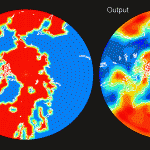
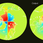
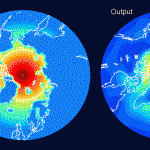
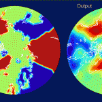
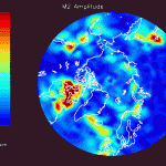
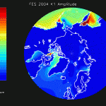
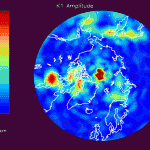
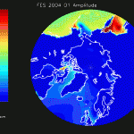
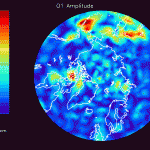
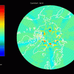
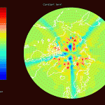
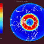
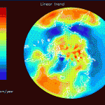
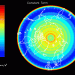
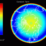
Arctic Ocean tides from GRACE (2007-11)
From 2007 to 2011, I used GRACE satellite acceleration data to recover Arctic ocean tides. My advisor Prof. John Wahr provided invaluable guidance, as did our colleagues from JPL: Dr. Shailen Desai, Dr. Dah-Ning Yuan and Dr. Michael Watkins.
Here’s the source code.
Abstract
Models are routinely used to remove the effects of global ocean tides from GRACE data during processing to reduce temporal aliasing into monthly GRACE solutions. These models have typically been derived using data from satellite altimeter missions such as TOPEX/Poseidon. Therefore the Arctic ocean components of tide models aren’t constrained by altimetry data, potentially resulting in errors that are likely to alias into monthly GRACE gravity fields at all latitudes.
Seven years of GRACE inter-satellite accelerations are inverted to solve for corrections to the amplitude and phase of major solar and lunar ocean tides at latitudes north of 50°N using a mascon approach. The tide model originally applied to our data was FES2004, truncated to maximum degree and order 90. Simulations are performed to verify that our inversion algorithm works as designed. Uncertainty estimates are derived from tidal solutions on land, and by subtracting two independent solutions that each use 3.5 years of data. Features in the M2, K1, S2, O1, and P1 solutions that rise above the noise floor likely represent errors in the FES2004 model. Errors due to truncating the spherical harmonic expansion of FES2004 are too small, and errors in the land mask model (needed to transform sea surface heights into mass) only affect coastal areas and don’t produce similar relative amplitudes for any examined tides. In the oceans north of 50°N, these residual estimates tend to reduce the FES2004 amplitudes for M2, K1, S2, O1, and P1.
The power spectra of accelerations are analyzed, and reductions in the variance of accelerations not used in our inversion suggest that our results can be used to improve GRACE processing.
Available Downloads
The source code is available. Also, here’s a quick link to browse the “control panel” of my code, followed by the top level of the program itself. All the functions used in that file are declared here and defined in full here.
This research is summarized in my dissertation, which is available as an electronic copy and a print copy. Here’s the presentation I gave at my defense.
I presented this research at the 2007, 2008, 2009, and 2010 AGU Fall Meetings. In 2011, it was published in JGR-Oceans (PDF) and highlighted in EOS.
1. Introduction
Earth’s gravity field varies both spatially and temporally. Gravity varies with time for many reasons including post-glacial rebound, hydrology, tides, and glacier thinning. Earth tides are relatively well modeled, but ocean tides aren’t as well understood because of the irregular drag and resonances caused by underwater bathymetry.
GRACE measures these gravity fluctuations using two satellites in the same low-earth orbit. One satellite (GRACE A) is ~220km ahead of the other satellite (GRACE B), and the two satellites are connected by a microwave ranging system that continuously measures their relative distance. Because the first satellite is ahead of the second, it’s affected by differences in local gravity before the second satellite. This delay can be used to deduce the underlying gravity variations. Many GRACE projects describe these gravity variations using spherical harmonics, but we chose to use mass concentrations (or “mascons”) to parameterize variations in local gravity.
A mass concentration located on the surface of the Earth can account for local gravity anomalies. The mascon’s mass can either be static in time, vary linearly or oscillate harmonically (or a linear combination of all these effects). A mascon’s mass can model tides by oscillating at semi-diurnal and diurnal tidal frequencies, or model hydrology by oscillating at semi-annual and annual frequencies.
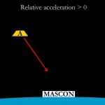
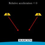
Our approach uses the relative accelerations between the GRACE satellites to solve for mascon values. The accelerations are smoothed using a CRN filter, and acceleration values measured in nm/s2 are available every 5 seconds. To illustrate a single mascon’s effect on GRACE accelerations, consider the case where one mascon lies directly beneath the GRACE satellites. In the following figures, red arrows represent the Newtonian force exerted on each satellite by the mascon.
Notice that a single, static mascon causes first weakly positive, then strongly negative, then weakly positive relative accelerations as GRACE flies over the mascon. The situation becomes more complicated when the mascon isn’t directly below the satellites. In figure 4, relative accelerations caused by a mascon in western Russia have been simulated as they would’ve been recorded by GRACE if the midpoint between the satellites was at any position on the map.
A single mascon causes significant relative accelerations even when the GRACE satellites are hundreds of kilometers away (in any direction). This means GRACE data can be used to recover semi-diurnal tides; the satellites don’t have to pass directly over a mascon twice within 12 hours to measure the semi-diurnal tide. GRACE’s second pass simply has to be close enough for that mascon’s effects to be measurable.
Even though figure 4 was produced by a single positive mascon, it appears very similar to the pattern one would expect from a single positive mascon with two negative mascons to the north and south. The positive accelerations to the north and south can cause an inversion algorithm to generate a “signal echo” where a single mascon generates two echoes of opposite sign to the north and south.
The fundamental measurement made by GRACE’s microwave ranging system is relative separation distance. Two time derivatives of this measurement are taken to provide relative acceleration, which reduces high frequency components and thus tends to limit spatial resolution. However, accelerations at any given time are determined solely by forces acting on the two satellites at that time, as opposed to separation distances/velocities which are determined by forces acting in the past. Inversion algorithms using acceleration don’t have to integrate gravitational forces over time. As a result, the computation time and hardware requirements are reduced compared to inversion algorithms using relative separation distances or velocities.
2. Simulations
To test the inversion algorithm, synthetic mascon fields were generated as inputs to a simulation. These mascons are separated by 230km and cover the Earth north of 50° N latitude. The synthetic mascon field included the following simultaneous time dependencies: constant, linear, M2 sine, M2 cosine, K1 sine, K1 cosine. These time dependencies have differing spatial patterns, designed to test the algorithm’s spatial resolution and ability to distinguish simultaneous frequencies.
Those input mascon fields (masses on the surface of the planet, measured in kg) were then “upward-continued” using Newtonian gravity to calculate the relative accelerations between the GRACE satellites caused by those mascon fields. The actual positions and times of the GRACE satellites over 5 years were used in this upward continuation process.
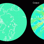
The resulting set of synthetic acceleration data was inverted using an algorithm that employs Newtonian gravity “in reverse” to deduce the surface mascon time dependencies. Thus a new “output” set of mascon fields are produced, which have the same units as the original synthetic mascon input fields. Here are the inputs and outputs of the simulations:
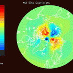
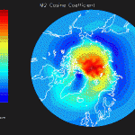
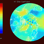
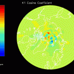
Notice that the sharp discontinuities in the M2 sine map (figure 7) don’t appreciably distort the M2 cosine map (figure 8). However, the K1 cosine map (figure 10) has anomalously high amplitudes near the north pole. This suggests that any large K1 amplitudes at the north pole aren’t real; the cause of this error is currently being investigated.
These simulations (and the real data inversions in the next section) were produced by adding a damping term to the covariance matrix which suppresses unphysically large fluctuations that otherwise dominate the maps.
In these simulations, the Newtonian gravity algorithm is applied twice, once for upward continuation from input field to synthetic acceleration time series, and once for inversion from acceleration time series to output mascon field. Also, instrumentation noise hasn’t yet been included.
3. Real Data Inversions
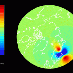
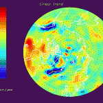
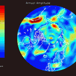
Real acceleration data provided by JPL were inverted to produce the following mascon fields:
Figure 11 confirms the post-glacial rebound in Canada and Scandinavia. It also confirms the secular trend associated with the melting glaciers in southeastern Greenland and Alaska. Figure 12 shows familiar hydrological signals which are again dominated by fluctuating glacier masses in Greenland and Alaska.
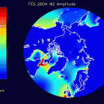
The acceleration data provided by JPL have already had FES 2004 and atmospheric tides removed. If these models were completely accurate, any attempt to solve for mascons with tidal oscillations would result in zero amplitude. However, if errors exist in FES 2004 which are proportional to the reported tide amplitude, one would expect areas with larger FES 2004 tide amplitudes to have larger residual mascon amplitudes. In other words, the output of the inversion should be large where FES 2004 is large, and small where FES 2004 is small (for instance, on land).
The figures that follow are grouped in pairs. On the left is FES 2004 for M2, K1, O1 and on the right is the corresponding residual amplitude from the mascon inversion.
In general, the residual maps have larger amplitudes in the ocean than on land, which supports the notion that ocean tides aren’t modeled as well as earth tides. Also, the largest amplitudes in the residual maps tend to be correlated with the largest amplitudes in the FES 2004 maps, reinforcing the idea that errors in FES are proportional to the amplitude.
4. Noise
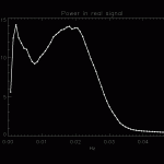
The relative acceleration time series can be sent through a Fast Fourier Transform to obtain a spectrum of the power at various frequencies:
Notice two distinct peaks, a sharp one centered on 0.003 Hz and a broader one at 0.02 Hz.
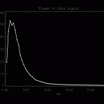
A synthetic mascon field with very large (and spatially short scale) amplitude fluctuations at many tidal frequencies and was upward continued to produce a synthetic noise spectrum:
This spectrum contains the most power at high frequencies that can reasonably be attributed to geophysical sources. As a result, power in the real data spectrum above f = 0.015 Hz probably isn’t geophysical in origin.
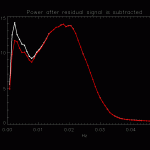
The real data inversions in section 3 should therefore be attempting to fit the signal in the first peak. To test this, the real data inversions were upward continued and subtracted from the original acceleration time series. Here is the resulting power spectrum:
Approximately 80% of the noise reduction of the first peak can be attributed to annual and linear parameters. The remaining noise reduction is due to the mascons’ oscillations at tidal frequencies M2, K1 and O1.
5. Conclusions
- Existing tide models such as FES 2004 have room for improvement.
- GRACE is a useful tool for recovering tidal signals even at semidiurnal frequencies.
- Errors in FES2004 aren’t significantly larger north of 66° N compared to south of 66° N (the TOPEX/Poseidon turning point).
- K1 simulations suggest that the large amplitudes near the north pole in the real inversion K1 maps aren’t caused by real signals.
Also, the authors would like to thank Fan-Chi Lin for his insightful comments regarding inversion approximations that eventually turned into the “zone of influence” algorithm described in the appendix.
6. Appendix: Algorithm Details
The inversion program is written in C++, compiles with g++ in Linux, and uses STL vectors and GSL routines. The resulting output was plotted using IDL. The source code will be released when it’s finished. Some custom algorithms in the program are described below: overlapping regions, zone of influence, and support grid points.
Overlapping regions
This program can’t simultaneously invert the entire region north of 50° N because of memory limitations; the covariance matrix scales as the square of the number of grid points. As a result, the grid is divided into “regions” which are solved independently. In other words, region 1 uses only the accelerations recorded when the satellites are over region 1 to solve exclusively for mascons inside region 1. This introduces the problem of boundary effects; mascons in region 2 that are near region 1 also influence the accelerations recorded in region 1 if those accelerations were recorded close enough to the mascons in region 2.
To avoid this problem, regions are split into two distinct parts. Each region has a central part which is directly adjacent to the central parts of nearby regions. The region also includes “overlap” around this central part, though. When that region is inverted, accelerations from the central and overlap parts of that region are used to solve for mascon amplitudes in the central and overlap parts of that region. The mascon amplitudes in the overlap parts are then discarded, and the mascon amplitudes from each region’s central part are combined to form the final map.
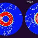
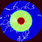
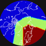
Here are the central and overlap parts of two regions. The central part is red while the overlap part of each region is green. Points that are completely outside the region are blue.
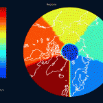
Notice that the red parts of each region don’t overlap, while the green parts do. Also, the second region can be larger than the first (polar) region because GRACE’s ground track density is higher at the poles. This causes polar regions to require more memory to solve for a given geographical area than non-polar regions. The central parts of each region can be shown on the same map:
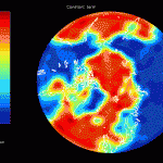
The extent to which boundary effects are reduced is determined by the size of the overlap part of each region. To test this reduction, a simulated signal (a constant 10 cm in oceans and 0 cm on land) was inverted once universally (i.e. without dividing the grid into regions) and using the regions shown in figure 24. Figure 25 shows the universal inversion, and figure 26 shows the difference between the universal inversion and the region inversion when the overlap is 1250 km. Figure 27 is the same as figure 26, but the overlap was set to 1850 km.
Notice that increasing the overlap distance decreases the difference (which can be assumed to be an error introduced by the overlapping region code). With the overlap set to 1250 km, large oscillations are observed near the north pole. Increasing the overlap to 1850 km reduces the size of these oscillations, but also reveals faint geometric lines at the region boundaries. Presumably larger overlap distances will eliminate these lines.
Zone of influence
The overlapping region code reduces the amount of memory required, but increases the computation time because the overlap parts of each region are calculated only to be thrown away. With computation times for high quality inversions measured in months on a quad core computer, a speedup was necessary. To accomplish this, the algorithm was re-written so each acceleration is only used to solve for mascons within a certain distance (measured from the mascon to the projection of the satellites’ midpoint onto the Earth’s surface).
In other words, as the satellites fly over the Earth they are assumed to only be influenced by mascons near them. This “zone of influence” moves with the satellites and is different for each acceleration, so in principle it’s necessary to calculate the distances from the satellites’ midpoint to all mascons at all times to determine which mascons lie within the zone of influence. Because there are millions of acceleration measurements, this strategy wouldn’t provide a speedup.
However, each acceleration value can be matched to the closest mascon (of which there are usually merely thousands rather than millions) and the zone of influence can be calculated using that mascon’s position rather than the position of the satellites’ midpoint. This approximation reduces the number of required calculations by a factor of 1000 and introduces negligible errors because any affected mascons are already far away from the acceleration measurement in question.
This algorithm has a single parameter– the zone of influence, measured in kilometers along the Earth’s surface. Smaller values dramatically reduce the computation time, but decrease the accuracy of the result by assuming that mascons can’t produce relative acceleration values when they’re outside the zone of influence surrounding the satellites. The simulated acceleration values in figure 4 suggest that choosing a zone of influence that’s too small to cover the non-zero portion of the map in figure 4 will lead to errors.
The simulations in section 2 and real inversions in section 3 used a zone of influence equal to 2850 km, and took 11 days to calculate. The following maps used an 850 km zone of influence, and finished in 4 hours:
The simulations with an 850 km zone of influence are considerably noisier and exhibit more signal echoing than the simulations in section 3 which used a 2850 km zone of influence.
Support grid points
One drawback of using Newtonian point mass gravity is that real tides are distributed over the surface of the earth rather than being concentrated as geometric points. This inaccuracy is usually avoided by modeling the mascons as disks using spherical harmonic expansions. These infinite series converge on a gravitational solution for a distributed mass, but their truncation introduces non-local errors.
These non-local errors can be circumvented by placing the point masses close enough together that GRACE isn’t sensitive enough to distinguish them. Unfortunately, this requires too much memory because the covariance matrix scales as the square of the number of grid points.
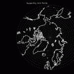
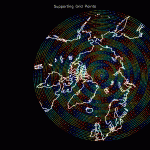
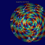
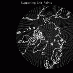
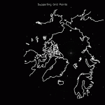
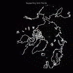
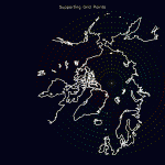
Our solution is to use “support grid points” to account for the distributed nature of the genuine water mass while avoiding non-local errors. Each “main grid point” has a set of support grid points associated with it. The support grid points fill the space between main grid points evenly, and can scale to create any desired density. Here are some examples, where main grid points are white and support grid points are colored differently based on which main grid point they’re associated with:
The support grid points’ gravitational effects are summed together (weighted according to surface area) with the main grid point to produce a single entry in the covariance matrix. In other words, support grid points don’t increase the memory requirements at all. (On the other hand, they don’t increase the spatial resolution of the resulting map either.) They allow the point mass algorithm to converge towards a representation of distributed masses while using a basis that doesn’t introduce non-local errors and is relatively fast compared to the spherical harmonic basis.
Surprisingly, the slowdown incurred by this code varies slower than linearly with respect to the number of added support grid points. This is due to the algorithm spending a large percentage of time in each loop calculating covariance matrix values (which are done after the support grid points are summed together and therefore doesn’t depend on them). The support points do slow down the calculation of Newtonian gravity for each mascon, but that calculation is comparatively quicker than the subsequent covariance matrix calculations which don’t depend on the number of support grid points at all.
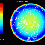
To test the support grid code, a constant 10 cm thickness of water was simulated over the entire surface (ocean and land) of the Earth north of 50° N latitude. This surface mass distribution was then upward-continued to obtain the relative accelerations as they would’ve been recorded by GRACE when the midpoint between the GRACE satellites was at any position on the map. This simulation was first performed by placing the mascons 100 km away from each other. Figure 37 shows the mascon distribution and figure 38 shows the relative accelerations due to the constant signal simulated by these mascons.
Notice that the relative accelerations are latitude-dependant, even though no such latitude dependence was programmed into the mascon field. This occurs because the mascon field doesn’t extend south of 50° N latitude. However, observe what happens when the mascons are placed 1050 km apart rather than 100 km apart:
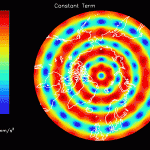
Significant fluctuations caused by the point mass approximation are visible. However, adding support grid points can improve the relative acceleration map by making it look more similar to figure 38. Start with 8 support points per main grid point:
This is an improvement, but better results can be obtained by assigning 24 support points to each grid point:
7. References
- Han, S.-C., Shum, C. K., and Matsumoto, K., 2005. GRACE observations of M2 and S2 ocean tides underneath the Filchner-Ronne and Larsen ice shelves, Antarctica. Geophysical Research Letters
- Lyard, F., Lefevre, F., Letellier, T., and Francis, O., 2006. Modelling the global ocean tides: modern insights from FES 2004. Ocean dynamics, 56:394-415
- Ray, R. D. and Luthcke, S. B., 2006. FAST TRACK PAPER: Tide model errors and GRACE gravimetry: towards a more realistic assessment. Geophysical Journal International
- Han, S.-C., Ray, R. D., and Luthcke, S. B., 2007. Ocean tidal solutions in Antarctica from GRACE inter-satellite tracking data. Geophysical Research Letters
- Moore, P. and King, M. A., 2008. Antarctic ice mass balance estimates from GRACE: Tidal aliasing effects. Journal of Geophysical Research (Earth Surface)
